

Uber's Billion Dollar Problem: Predicting ETAs Reliably And Quickly
Uber's Billion Dollar Problem: Predicting ETAs Reliably And Quickly
A visual deep dive into how Uber uses graph theory, embeddings and self-attention and to predict ETAs

Get a list of personally curated and freely accessible ML, NLP, and computer vision resources for FREE on newsletter sign-up.
To read more on this topic see the references section at the bottom. Consider sharing this post with someone who wants to know more about machine learning.

Imagine you have a flight to catch in an hour, and you're relying on Uber to get you to the airport. An accurate Estimated Time of Arrival or ETA allows you to relax, knowing exactly how much time you have. In contrast, an unreliable ETA can be a recipe for stress, leaving you scrambling to hail another cab or risk missing your flight.
For Uber, accurate ETAs are crucial not just for user experience, but also for their bottom line. Imagine a scenario where riders consistently experience delays due to inaccurate ETAs. This can lead to frustration and a decrease in ridership, impacting Uber's revenue.
0. Why is predicting ETA so important?
Predicting an accurate Estimated Time of Arrival or ETA is crucial for Uber's success. Inaccurate ETAs can result in a poor user experience, leading to decreased usage and lost earnings [4].
This directly affects the company's earnings, resulting in a loss of millions of dollars over a few weeks in just a few cities. Extrapolating this to all of Uber's operational countries would result in a substantial financial loss of billions of dollars [4].
Further, Uber's ETA prediction service is used by internal products and helps allocate resources efficiently. During a ride, the ETA service shows the user the time to destination, dispatches the best car to minimize wait time, and takes the user from source to destination, updating ETA multiple times.
1. Uber’s Design Decisions
In the past, Uber used gradient-boosted decision tree ensembles to predict ETAs. With the increasing amount of training data available with time, it was only natural to scale to more powerful machine learning models.
Uber decided to switch from decision tree ensembles to deep learning models. Switching to models closer to state-of-the-art meant they would need to solve problems that come with scaling to such models. Uber designed the ML system with the following constraints [2] in mind:
Latency: The ETA prediction ML model has the highest queries per second at Uber. It needs to scale and be a low-latency service used by internal Uber customers.
Accuracy: Uber's primary metric is the mean absolute error (MAE) between predicted ETA and true ETA. The new ML model must improve over the XGBoost model.
Generalizable: Uber’s model must provide reliable ETA predictions across Uber’s countries and different business cases such as Uber Eats and Uber Rides
2. Don’t Reinvent The Wheel
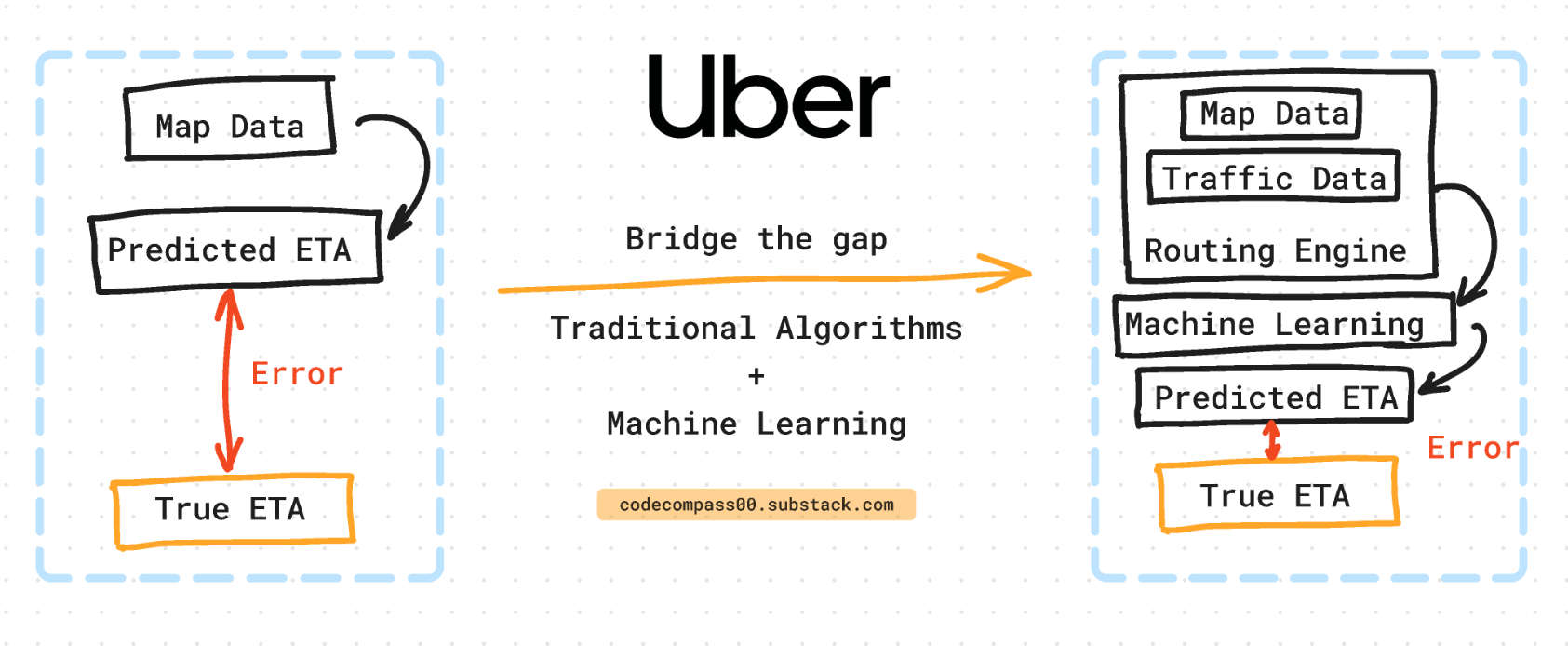
Uber's ETA system is a clever marriage of traditional routing algorithms and cutting-edge deep learning. Think of it like a layered cake. The first layer is a routing engine that uses map data, traffic patterns, and vehicle speeds to create a basic estimate of travel time.
But the real magic happens on top of this foundation. Here, Uber utilizes a deep learning model that learns from vast amounts of real-world data to account for subtle factors like time of day, weather conditions, and even driver behavior. This allows Uber to refine the initial estimate and provide a much more accurate ETA.

Graph Theory and Dijkstra To The Rescue
Instead of throwing all prior know-how about traffic and routing out of the window and starting from the ground up, they solve it by standing on the shoulders of giants.
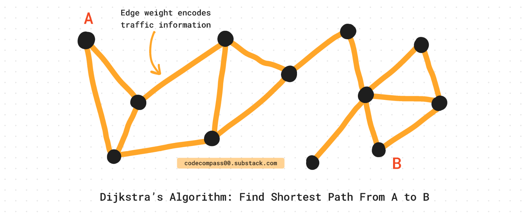
Uber uses “plain-old”, not-so-exciting-as-deep-learning graph theory and shortest path algorithms like Dijkstra’s [12] to solve the problem. Graph theory is well studied and using classical algorithms reliably brings the predicted ETA much closer to the true ETA. It uses map data, distances, and vehicle speed. But it misses a lot of nuances of what it means to drive from location A to B.
Lightweight ML Model
Adding a layer of machine learning to the existing engine improves ETA prediction by accounting for real-world variables such as time of day, weather, and location. The ML model can learn and predict subtle nuances that impact ETA.
The machine learning model is laid on top of a priori modeling of traffic and routing. The ML model’s goal is to predict the residual between the routing engine and the true ETA.
A by-product of this design is that the routing engine is isolated from the ML model. This allows Uber to independently fine-tune and update the machine-learning model without touching the routing engine.
3. Uber’s Routing Engine
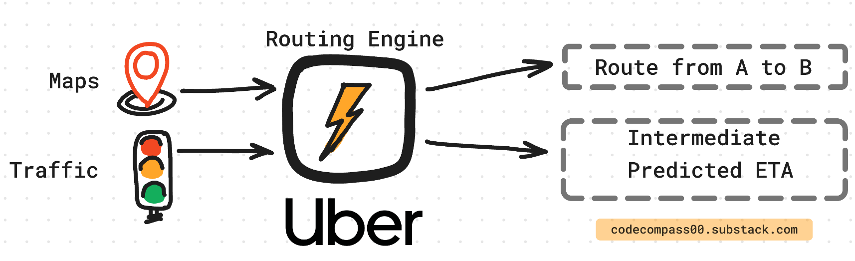
What is routing?
Problem statement: Given a source A and destination B:
Find a feasible route from A to B.
Predict the time taken to make the trip from A to B = predict ETA.
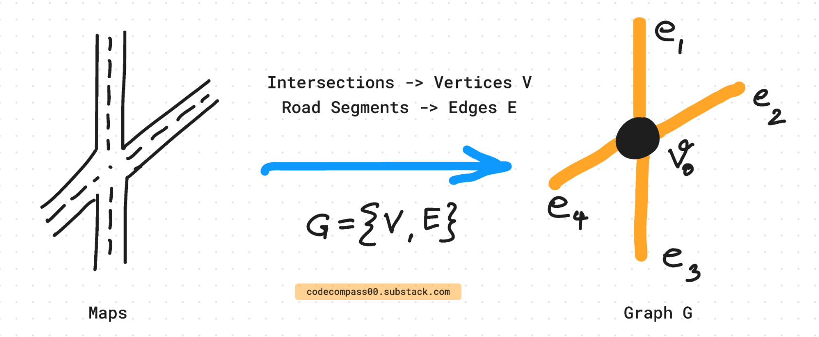
This process involves modeling the city as a graph, where each road segment is an edge and each intersection is a node.
To find the shortest path between points A and B, Dijkstra's algorithm can be used, which has a time complexity of O(N log N), where N is the number of nodes in the graph. In the case of San Francisco's Bay Area, there are approximately 500,000 nodes, and the ETA prediction service receives 500,000 requests per second.
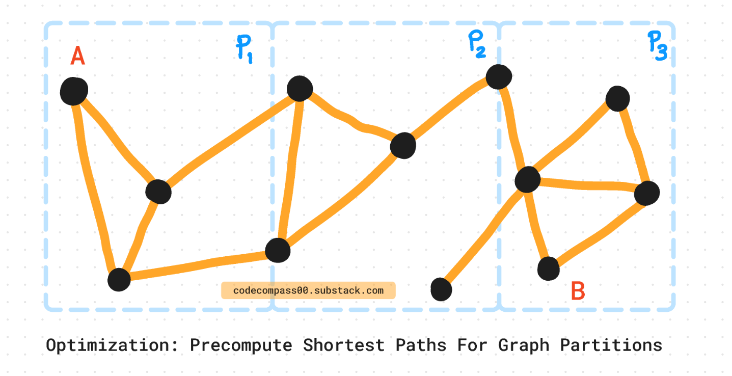
Divide and Conquer: Partitioning Algorithm
Divide the city into partitions and pre-compute the shortest parts of each partition. This means at query time, Uber only needs to compute the shortest path that lies on the perimeter of these partitions. This pre-computation reduces the complexity of each partition from N to sqrt(N).
Traffic Modeling
Traffic is a function of real-time events such as the time of the day, whether is there a concert happening nearby, what is the weather outside, etc.
GPS data from vehicles is used to model the traffic on a particular road segment between points A and B. This is done by accumulating real data over the segment and calculating the “speed” across the road segment between A and B. This is distance(A, B) / time_taken(A, B).
The routing algorithm is made aware of the traffic by providing weights to each road segment edge. The weight value determines whether the segment has high traffic or low traffic.
4. Converting Features To Embeddings
Uber bins both categorical and continuous-valued features. These are then embedded in D-dimensional space. Bucketing continuous values based on quantiles is counter-intuitive but shows empirical improvement [7] through their experiments.
One explanation is that for any fixed number of buckets, quantile buckets convey the most information in bits about the original feature value compared to any other bucketing scheme. [7]
Geospatial information such as the source or destination (longitude, latitude) is encoded differently using Geohash [11]. Most regions on the globe have varying density, Uber also has more data points for certain points than others. Instead of a fixed grid system, Uber quantizes the globe based on density. Regions like New York City and Bengaluru are allowed much higher spatial resolution than more remote regions.
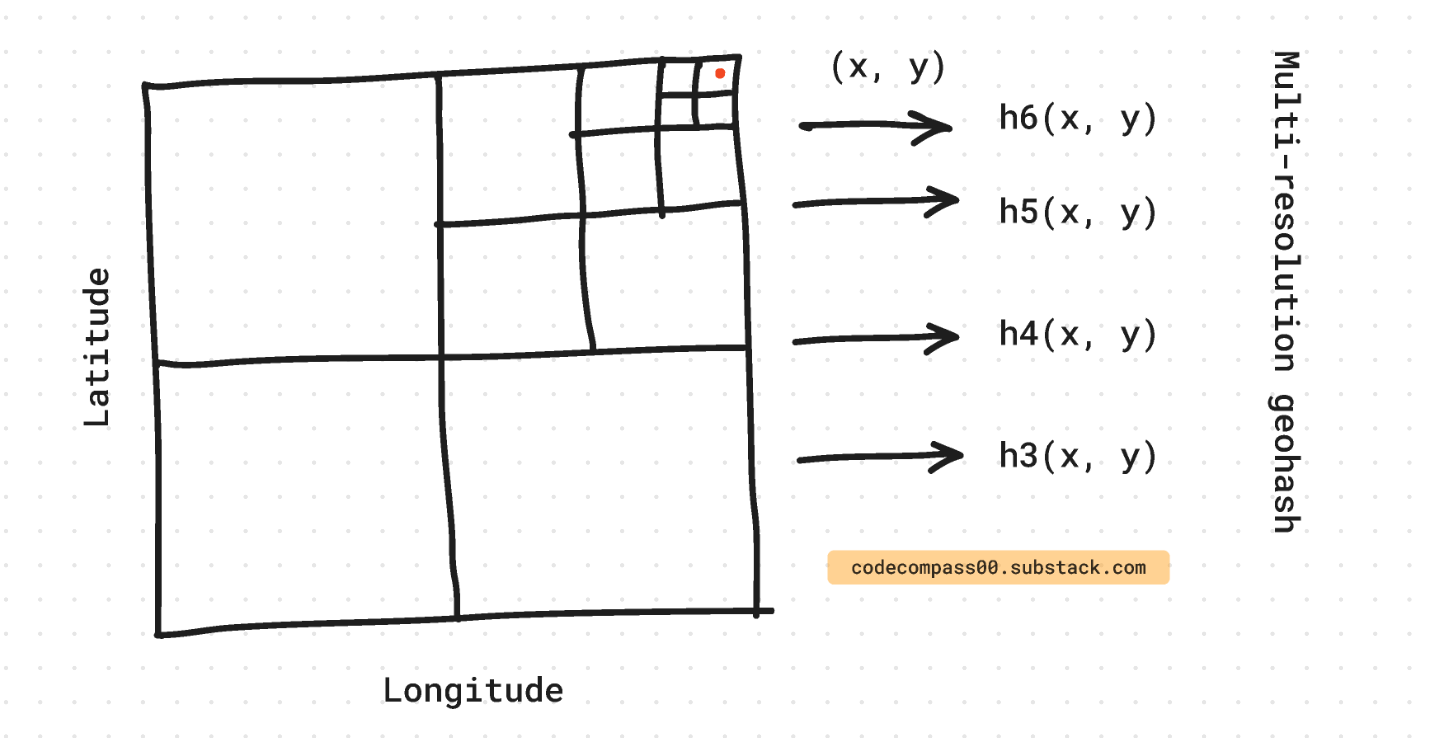
To trade-off between space constraints and precision, Uber uses multi-resolution hashing. This way the glob is divided at R different resolutions. For any location on the map, R different feature vectors are concatenated to produce the feature vector for that location.
5. 2-Layer Model Architecture
Uber experiments concluded that an encoder-decoder architecture with self-attention provided the lowest error. Uber experimented with 7 different neural network architectures. This included MLPs [3], TabNet [6], mixture-of-experts [6], and transformers [1].
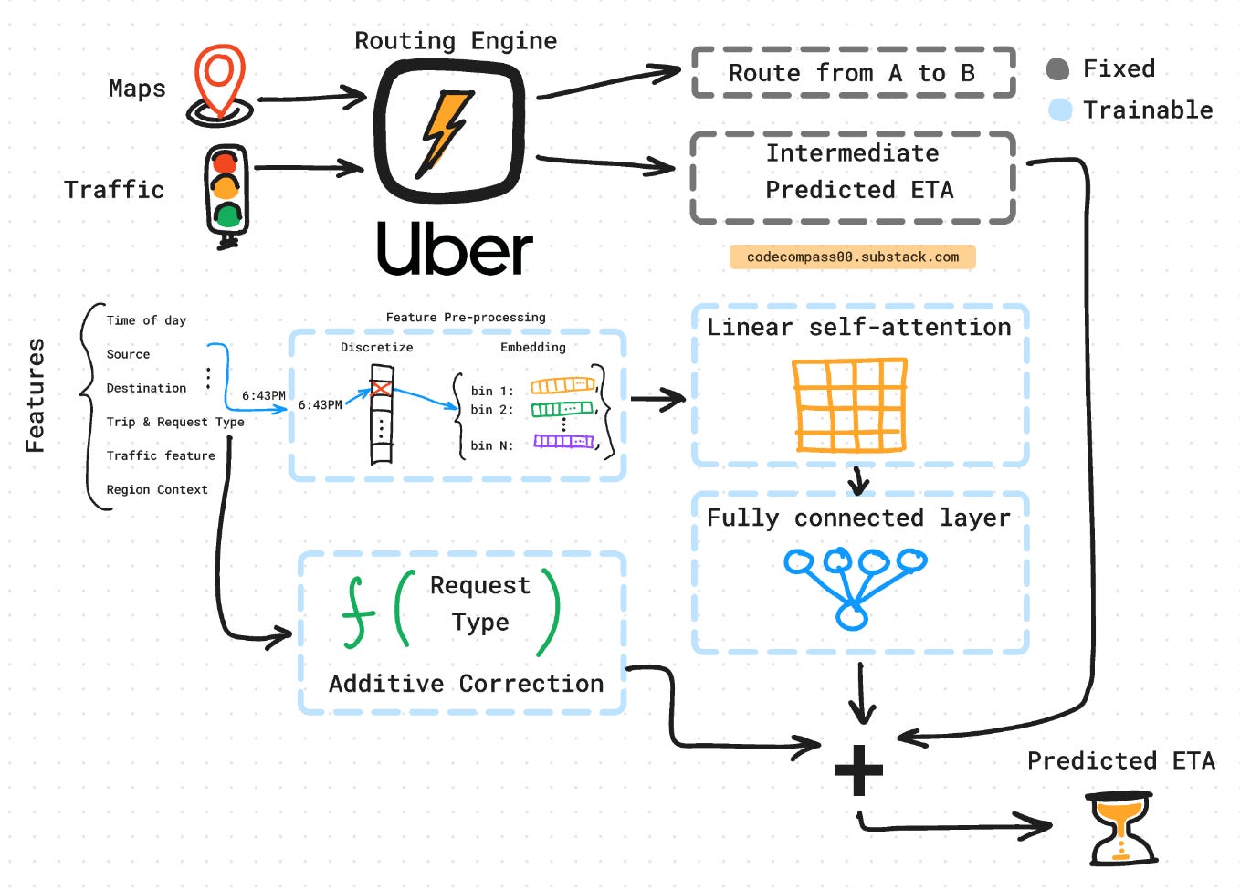
The output of the routing engine and embedded features are used as input to the model. For efficiency, the input features are discretized with their corresponding embeddings. The model takes these and outputs the residual ETA. Finally, a calibration layer is used to offset the prediction depending on the type of request made to the ETA prediction service.
Encoder-Decoder Architecture
To keep the model lightweight it is “shallow” with 2 layers. 99% of the parameters are in the form of embedding lookup tables [7]. Uber discretizes continuous values into separate bins and learns different embeddings for each bin. This means only relevant a fraction of the lookup tables are queried for a single point.
With the quantization as binning is a hash, it costs O(1) to look up the embeddings table. On the other hand, looking up a tree structure would cost O(log N), or even more expensive would be to use a fully connected layer to project the features.
The model output is passed through ReLU to ensure positive ETA times and clamping to prevent extreme values. An offset adjuster or bias is added on top of the model to further tune the model based on downstream tasks.
Self-Attention on Tabular Data
Vision and language models use self-attention to capture dependencies given an input sequence. In Uber’s case, the sequence is all the relevant information such as the time of day, source A, destination B, distance between A and B, etc. In language, the order of these pieces matters, however, in Uber’s case there is no notion of a sequence, so they drop the positional encoding.
The self-attention layer takes as input K pieces of information. For each piece, it looks at all K pieces for clues and outputs a re-weighted piece. For K pieces of information, self-attention produces a K x K attention matrix.
The self-attention mechanism rescales to give less or more importance to information based on other pieces of information. For example, the distance between A and B can be given high importance when the model realizes that it is a rush hour with peak traffic based on time of day and traffic information.
To speed up and meet the latency requirements, the linear transformer [8] is used to reduce complexity from the vanilla transformer O(K^2) to O(K). Since, K > D, using the linear transformer is more efficient.
Loss Function
Uber uses a variant of the robust Huber loss [9]: the asymmetric Huber loss [7].
By varying omega, you can control the relative cost of underprediction vs overprediction, which is useful in situations where being a minute late is worse than being a minute early. [2]
Huber loss is well known for robust regression [10] and can be tuned to control sensitivity to outliers.
6. Reliable ETA Predictions Across Data Distributions
Based on what kind of downstream task is using the ETA predictor service, offset or bias adjustment is made depending on the use case. This improves accuracy as use cases across different countries, long vs. short trips, etc., all have different error distributions.
ETA error distribution in different locations is different. India has a thicker long-tail distribution compared to North America, meaning there are more observations of really large ETA errors in India than in NA.
The ML model captures these nuances not just in the region of operation but also in time of day, driver behavior, traffic, etc.
The ETA is highly non-linear with variables such as time of day and it is difficult to have priors on this interaction. Uber relies on data-driven, non-parametric models to predict non-linear interactions between inputs and the output: ETA.
7. Periodic Automatic Retraining and Fallback Mechanisms
Uber has internal services to collect fresh data, re-train, validate, and automatically deploy newly trained ML models to their services.
Uber continuously monitors ETA services and places fallback mechanisms to replace the main service when it breaks. This ensures that downstream users of the ETA prediction service can function even during downtimes.
Consider subscribing to get it straight into your mailbox:
Continue reading more:


References
[1] Attention Is All You Need: https://arxiv.org/abs/1706.03762
[2] DeepETA: https://www.uber.com/en-GB/blog/deepeta-how-uber-predicts-arrival-times/
[3] MLP: https://en.wikipedia.org/wiki/Multilayer_perceptron
[5] TabNet: Attentive Interpretable Tabular Learning: https://arxiv.org/abs/1908.07442
[6] Outrageously Large Neural Networks: The Sparsely-Gated Mixture-of-Experts Layer: https://arxiv.org/abs/1701.06538
[7] DeeprETA: An ETA Post-processing System at Scale: https://arxiv.org/abs/2206.02127
[8] Transformers are RNNs: Fast Autoregressive Transformers with Linear Attention: https://arxiv.org/abs/2006.16236
[9] Huber Loss: https://en.wikipedia.org/wiki/Huber_loss
[10] Robust Regression: https://en.wikipedia.org/wiki/Robust_regression
[11] Geohash: https://en.wikipedia.org/wiki/Geohash
[12] Dijkstra's Algorithm: https://en.wikipedia.org/wiki/Dijkstra's_algorithm
Consider sharing this newsletter with somebody who wants to learn about machine learning:
this newsletter looks very familiar, interesting.